Quantum Neural Network Get Started

Content

1. Quantum Neural Network Overview
2. Quantum Neural Network Data Loading
3. Quantum Neural Network Forward
4. Quantum Neural Network Backward
5. TwoLayerQNN

1. Quantum Neural Network Overview

A typtical quantum neural network includes four steps:

• Step 1: Encode the classical data into a quantum state

• Step 2: Apply a parameterized model

• Step 3: Measure the circuit to extract labels

• Step 4: Use optimization techiiques to update model parameters

Before we dig into the details, we first clarity several concepts:

1.1 What is parameterized model

Parameterized circuit has three names:

• Parameterized quantum circuit
• Ansatz
• Variational Circuit

All of them refer to the same thing, which is a circuit that contains some variational paramters.

2. Quantum Neural Network Data Loading

We introduce three methods to encode data:

2.1 Basis encoding

This refers to encode data into computational basis states.

For example, if \(x_{1} = 01\) and \(x_{2} = 10\), we can use a two-qubit quantum state that is a superposition of state \(\vert 01 \rangle\) and \(\vert 10 \rangle\).

2.2 Amplitude Encoding

This refers to encode data into amplititudes.

For example, if a vector is \([1,1,0,1]\), we can use a two-qubit quantum state that is a superposition of state \(\vert 00\rangle\), \(\vert 01\rangle\), \(\vert 11\rangle\) with equal weights.

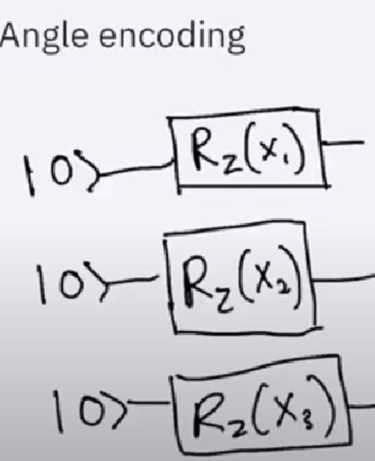
2.3 Angle Encoding

This refers to encode data into rotation angle. We can see the following figure that encodes \(x_{1}\), \(x_{2}\), \(x_{3}\) on the circuit.

3. Quantum Neural Network Forward

We combine Qiskit to explain how neural network forwards to the final cost function.

The following circuit uses a Hardmard gate, followed by a Rotation-Y and Rotation-X. The input and weight is encoded as angle to these two operations.

We then introduce Cost function to the circuit. The tutorial use a PauliSUmOp as the cost function, which means the Z and X operator will be used as the measurement operator to the final result. Both operator will times 1 and add together.

# construct cost operator
H1 = StateFn(PauliSumOp.from_list([("Z", 1.0),("X", 1.0)]))

We will get the expectation value of neural network cost.

The overall circuit construction looks like the following:

import numpy as np

from qiskit import Aer, QuantumCircuit
from qiskit.circuit import Parameter
from qiskit.circuit.library import RealAmplitudes, ZZFeatureMap
from qiskit.opflow import StateFn, PauliSumOp, AerPauliExpectation, ListOp, Gradient
from qiskit.utils import QuantumInstance, algorithm_globals
from qiskit_machine_learning.neural_networks import OpflowQNN

algorithm_globals.random_seed = 42

# set method to calculcate expected values
expval = AerPauliExpectation()

# define gradient method
gradient = Gradient()

# define quantum instances (statevector and sample based)
qi_sv = QuantumInstance(Aer.get_backend("aer_simulator_statevector"))

# we set shots to 10 as this will determine the number of samples later on.
qi_qasm = QuantumInstance(Aer.get_backend("aer_simulator"), shots=10)

# construct parametrized circuit
params1 = [Parameter("input1"), Parameter("weight1")]
qc1 = QuantumCircuit(1)
qc1.h(0)
qc1.ry(params1[0], 0)
qc1.rx(params1[1], 0)
qc_sfn1 = StateFn(qc1)

# construct cost operator
H1 = StateFn(PauliSumOp.from_list([("Z", 1.0), ("X", 1.0)]))

# combine operator and circuit to objective function
op1 = ~H1 @ qc_sfn1
print(op1)

# construct OpflowQNN with the operator, the input parameters, the weight parameters,
# the expected value, gradient, and quantum instance.
qnn1 = OpflowQNN(op1, [params1[0]], [params1[1]], expval, gradient, qi_sv)

Now let’s test some parameters to see how it functions.

Case 1: input = 0, weight = 0

input1 = np.array([0])
weights1 = np.array([0])
# Use Aer's qasm_simulator
simulator = QasmSimulator()
#reproduce the circuit
qc1 = QuantumCircuit(1)
qc1.h(0)
qc1.ry(input1[0], 0)
qc1.rx(weights1[0], 0)
qc1.save_statevector() # Save statevector
qobj = assemble(qc1)
state = sim.run(qobj).result().get_statevector() # Execute the circuit
print(state)        
Result: [0.70710678+0.j 0.70710678+0.j] 

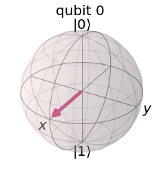
Here we get a qubit’s statevector instead of the Bloch vector. The state vector is

THe bloch vector is shown in the below figure:

As you can see, the bloch vector is

Now, we need to consider what is the cost value now?

The cost is a sum of two operators Z and X.

We think from a projection perspective, \([1,0,0]\) has projection on Z with value of 0 and has projection on X with value of 1. The final result should be 1.

Let’s verify it.

# QNN batched forward pass
qnn1.forward(input1, weights1)
array([[1.]])

The result is exactly 1. But if we think from state vector, we may not be able to get 1 easily.

Case 2: Input = 2/pi, weight = 0

input1 = np.array([np.pi/2])
weights1 = np.array([0])
# Use Aer's qasm_simulator
simulator = QasmSimulator()
#reproduce the circuit
qc1 = QuantumCircuit(1)
qc1.h(0)
qc1.ry(input1[0], 0)
qc1.rx(weights1[0], 0)
qc1.save_statevector() # Save statevector
qobj = assemble(qc1)
state = sim.run(qobj).result().get_statevector() # Execute the circuit
print(state)
[0.+0.j 1.+0.j]         

Neural Network Forward - result:

# QNN batched forward pass
qnn1.forward(input1, weights1)
array([[-1.]])

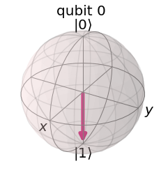
We also draw the bloch sphere here:

The bloch vector is \([0,0,-1]\)

With the same projection idea, we can know the cost is -1.

Now we know how neural network forwards and we can compute the exact cost value by ourselves.

4. Quantum Neural Network Backward

Quantum neural network uses parameter shift method to compute gradient.

4.1 Pauli gate example

Consider a quantum computer with parameterized gates of the form \(U_{i}\left(\theta_{i}\right)=\exp \left(-i \frac{\theta_{i}}{2} \hat{P}_{i}\right),\) where \(\hat{P}_{i}=\hat{P}_{i}^{\dagger}\) is a Pauli operator.

The gradient of this unitary is \(\nabla_{\theta_{i}} U_{i}\left(\theta_{i}\right)=-\frac{i}{2} \hat{P}_{i} U_{i}\left(\theta_{i}\right)=-\frac{i}{2} U_{i}\left(\theta_{i}\right) \hat{P}_{i}\)

Substituting this into the quantum circuit function \(f(x ; \theta)\), we get \(\begin{aligned} \nabla_{\theta_{i}} f(x ; \theta) &=\frac{i}{2}\left\langle\psi_{i-1}\left|U_{i}^{\dagger}\left(\theta_{i}\right)\left(P_{i} \hat{B}_{i+1}-\hat{B}_{i+1} P_{i}\right) U_{i}\left(\theta_{i}\right)\right| \psi_{i-1}\right\rangle \\ &=\frac{i}{2}\left\langle\psi_{i-1}\left|U_{i}^{\dagger}\left(\theta_{i}\right)\left[P_{i}, \hat{B}_{i+1}\right] U_{i}\left(\theta_{i}\right)\right| \psi_{i-1}\right\rangle \end{aligned}\) where \([X, Y]=X Y-Y X\) is the commutator. We now make use of the following mathematical identity for commutators involving Pauli operators (Mitarai et al. (2018)): \(\left[\hat{P}_{i}, \hat{B}\right]=-i\left(U_{i}^{\dagger}\left(\frac{\pi}{2}\right) \hat{B} U_{i}\left(\frac{\pi}{2}\right)-U_{i}^{\dagger}\left(-\frac{\pi}{2}\right) \hat{B} U_{i}\left(-\frac{\pi}{2}\right)\right)\)

Substituting this into the previous equation, we obtain the gradient expression \(\begin{aligned} \nabla_{\theta_{i}} f(x ; \theta)=& \frac{1}{2}\left\langle\psi_{i-1}\left|U_{i}^{\dagger}\left(\theta_{i}+\frac{\pi}{2}\right) \hat{B}_{i+1} U_{i}\left(\theta_{i}+\frac{\pi}{2}\right)\right| \psi_{i-1}\right\rangle \\ &-\frac{1}{2}\left\langle\psi_{i-1}\left|U_{i}^{\dagger}\left(\theta_{i}-\frac{\pi}{2}\right) \hat{B}_{i+1} U_{i}\left(\theta_{i}-\frac{\pi}{2}\right)\right| \psi_{i-1}\right\rangle \end{aligned}\)

Finally, we can rewrite this in terms of quantum functions: \(\nabla_{\theta} f(x ; \theta)=\frac{1}{2}\left[f\left(x ; \theta+\frac{\pi}{2}\right)-f\left(x ; \theta-\frac{\pi}{2}\right)\right]\)

5. TwoLayerQNN

Now we start to construct a more complex quantum neural network.

from qiskit_machine_learning.neural_networks import TwoLayerQNN
# specify the number of qubits
num_qubits = 3
# specify the feature map
fm = ZZFeatureMap(num_qubits, reps=2)
fm.draw(output="mpl")

# specify the ansatz
ansatz = RealAmplitudes(num_qubits, reps=1)
ansatz.draw(output="mpl")

# specify the observable
observable = PauliSumOp.from_list([("Z" * num_qubits, 1)])
print(observable)

5.1 ZZFeatureMap

We first need to understand ZZFeatureMap.

ZZFeatureMap embedding \(n\)-dimensional classical data on \(n\) qubits: \(U_{\phi(x)} H^{\otimes n}\), where \(\begin{gathered} U_{\phi(x)}=\exp \left(i \sum_{S \subseteq[n]} \phi_{S}(x) \prod_{i \in S} Z_{i}\right) \\ \phi_{i}(x)=x_{i}, \phi_{\{i, j\}}(x)=\left(\pi-x_{0}\right)\left(\pi-x_{1}\right) \end{gathered}\) and \(Z_{i}\) is a \(Z\)-gate on the \(i\)-th qubit.

**ZZFeatureMap is using RZ operator to transfer input data into a higher dimension data. **

Considering the 2-dimensional, 2-qubit case, \(U_{\phi(x)}=\exp \left(i x_{0} Z_{0}+i x_{1} Z_{1}+i\left(\pi-x_{0}\right)\left(\pi-x_{1}\right) Z_{0} Z_{1}\right)\)

The first \(2 U 1\) rotations is that since \(\exp (i \theta Z)=R Z(2 \theta)\) up to global phase and \(R Z\) is equivalent to \(U 1\) up to global phase, we might as well use \(U 1\left(2 \phi_{i}(x)\right)\). Is that correct?

Then how do we then get \(C X U 1\left(2 \phi_{\{0,1\}}(x)\right) C X\) from \(\exp \left(i \phi_{\{0,1\}}(x) Z_{0} Z_{1}\right)\) ?

By the definition of \(U 1(\lambda)\) in qiskit, it is equivalent to \(R Z\) up up a phase factor. Now note that: \(Z_{0} Z_{1}=Z \otimes Z=\left(\begin{array}{cc} 1 & 0 \\ 0 & -1 \end{array}\right) \otimes\left(\begin{array}{cc} 1 & 0 \\ 0 & -1 \end{array}\right)=\left(\begin{array}{cccc} 1 & 0 & 0 & 0 \\ 0 & -1 & 0 & 0 \\ 0 & 0 & -1 & 0 \\ 0 & 0 & 0 & 1 \end{array}\right)\)

since this is diagonal, we have that \(e^{-i \lambda Z_{0} Z_{1}}=\left(\begin{array}{cccc} e^{-i \lambda} & 0 & 0 & 0 \\ 0 & e^{i \lambda} & 0 & 0 \\ 0 & 0 & e^{i \lambda} & 0 \\ 0 & 0 & 0 & e^{-i \lambda} \end{array}\right)=\left(\begin{array}{cc} R_{Z}(2 \lambda) & \mathbf{0} \\ \mathbf{0} & X R_{Z}(2 \lambda) X \end{array}\right)\) since $$X R_{Z}(2 \lambda) X=\left(\begin{array}{cc}0 & 1 \ 1 & 0\end{array}\right)\left(\begin{array}{cc}e^{-i \lambda} & 0 \ 0 & e^{i \lambda}\end{array}\right)\left(\begin{array}{cc}0 & 1 \ 1 & 0\end{array}\right)=\left(\begin{array}{cc}e^{i \lambda} & 0 \ 0 & e^{-i \lambda}\end{array}\right)$

Thus, to implement \(e^{-i \lambda Z_{0} Z_{1}}\) we would have a circuit like: Note that this circuit can be written as \(C X \cdot\left(I \otimes R_{Z}\right) \cdot C X\). Also by knowing this, you can check this explicitly as well, by first note that \(\otimes R_{Z}(2 \lambda)=\left(\begin{array}{cc} 1 & 0 \\ 0 & 1 \end{array}\right) \otimes\left(\begin{array}{cc} e^{-i \lambda} & 0 \\ 0 & e^{i \lambda} \end{array}\right)=\left(\begin{array}{cccc} e^{-i \lambda} & 0 & 0 & 0 \\ 0 & e^{i \lambda} & 0 & 0 \\ 0 & 0 & e^{-i \lambda} & 0 \\ 0 & 0 & 0 & e^{i \lambda} \end{array}\right)\)

then \(C X \cdot(I \otimes R Z(2 \lambda)) \cdot C X\) is equal to \(\begin{aligned} \left(\begin{array}{llll} 1 & 0 & 0 & 0 \\ 0 & 1 & 0 & 0 \\ 0 & 0 & 0 & 1 \\ 0 & 0 & 1 & 0 \end{array}\right) &\left(\begin{array}{cccc} e^{-i \lambda} & 0 & 0 & 0 \\ 0 & e^{i \lambda} & 0 & 0 \\ 0 & 0 & e^{-i \lambda} & 0 \\ 0 & 0 & 0 & e^{i \lambda} \end{array}\right)\left(\begin{array}{llll} 1 & 0 & 0 & 0 \\ 0 & 1 & 0 & 0 \\ 0 & 0 & 0 & 1 \\ 0 & 0 & 1 & 0 \end{array}\right) \\ &=\left(\begin{array}{cccc} e^{-i \lambda} & 0 & 0 & 0 \\ 0 & e^{i \lambda} & 0 & 0 \\ 0 & 0 & e^{i \lambda} & 0 \\ 0 & 0 & 0 & e^{-i \lambda} \end{array}\right) \end{aligned}\)

5.2 RealAmplititude

The RealAmplititude circuit consists of of alternating layers of rotations Y and entanglements CX. The entanglement pattern can be user-defined or selected from a predefined set. It is called RealAmplitudes since the prepared quantum states will only have real amplitudes, the complex part is always 0.

The real-amplitude builds two-local circuit.

5.3 The two-local circuit

The two-local circuit is a parameterized circuit consisting of alternating rotation layers and entanglement layers. The rotation layers are single qubit gates applied on all qubits. The entanglement layer uses two-qubit gates to entangle the qubits according to a strategy set using entanglement.

quantum circuit that has N qudits is said to be n-local if the gates act nontrivially on at most nn-qudits with n≤Nn≤N. As an example, here is a circuit of non-trivial gates acting on at most 2-qubits in a system of 3-qubits.

5.4 Why we use two-local circuit as Anastz

If we want to get some eigenstate by optimization, we need to present these eigenstates. Most eigenstates are entangled.

Here is an example to see why you need to be able to generate entangle state to have successful VQE calculation, supposed you have the Hamiltonian $$H=\left(\begin{array}{llll}0 & 0 & 0 & 1 \ 0 & 0 & 1 & 0 \ 0 & 1 & 0 & 0 \ 1 & 0 & 0 & 0\end{array}\right)$

And you running VQE to find the lowest eigenvalue to this Hamiltonian. This means you need to be able to generate the eigenstate that correspond to the lowest eigenvalue. Now, if you look at all the eigenstates of \(H\) and their correspondence eigenvalues:

Here you should notice that these states are all entangled. So if we want to use the algorithm to find the lowest eigenvalue \((-1)\) in this case, it must be able to generate an entangled state.

To summary, entanglement is neccessary in some cases.

5.5 Overall Circuit

from qiskit_machine_learning.neural_networks import TwoLayerQNN
# specify the number of qubits
num_qubits = 3
# specify the feature map
fm = ZZFeatureMap(num_qubits, reps=2)

# specify the ansatz
ansatz = RealAmplitudes(num_qubits, reps=1)

# specify the observable
observable = PauliSumOp.from_list([("Z" * num_qubits, 1)])

# define two layer QNN
qnn3 = TwoLayerQNN(
    num_qubits, feature_map=fm, ansatz=ansatz, observable=observable, quantum_instance=qi_sv
)

# define (random) input and weights
input3 = algorithm_globals.random.random(qnn3.num_inputs)
weights3 = algorithm_globals.random.random(qnn3.num_weights)

# QNN forward pass
qnn3.forward(input3, weights3)

# QNN backward pass
qnn3.backward(input3, weights3)

Reference:

1. Nielsen, Michael A., and Isaac Chuang. "Quantum computation and quantum information." (2002): 558-559.

2. Qiskit Quantum Neural Network Tutorial (https://qiskit.org/documentation/machine-learning/tutorials/01_neural_networks.html)

3. Parameter Shift from Pennylane: https://pennylane.ai/qml/glossary/parameter_shift.html

4. ZZFeatureMap Explaination: https://quantumcomputing.stackexchange.com/questions/17868/quantum-circuit-for-the-zz-feature-map

5. Why we need entaglement in Anastz: https://quantumcomputing.stackexchange.com/questions/17585/role-of-entanglement-in-a-vqe-ansatz-for-combinatorial-problems

6. TwoLocal Source Library: https://qiskit.org/documentation/stubs/qiskit.circuit.library.TwoLocal.html

7. RealAmplititude Source Lirbary: https://qiskit.org/documentation/stubs/qiskit.circuit.library.RealAmplitudes.html