Content
- QAE Algorithm
- Maximum Likelihood Estimation
- QAE + MLE
- Expectation Value Computation
- Option Pricing Scenario
QAE Algorithm
1. Review of Grover Search
The amplitude amplification operator \(\vert \Psi\rangle=\mathcal{A}\vert 0\rangle=\left\vert \Psi_{1}\right\rangle+\left\vert \Psi_{0}\right\rangle .\)
- \(U_{\chi}\) is the oracle function: \(\vert x\rangle \longmapsto\left\{\begin{aligned}-\vert x\rangle & \text { if } \chi(x)=1 \\\vert x\rangle & \text { otherwise } \end{aligned}\right.\)
In this equation, \(\mathcal{A}\) helps to transfer \(\vert 0\rangle\) to state \(\vert\Psi_{0}\rangle\).
- The amplitude amplification operator is: \(Q=\left(\mathcal{A}(2\vert 0\rangle\langle 0\vert -I) \mathcal{A}^{\dagger}\right) \times U_{\chi}\)

Now we try to infer
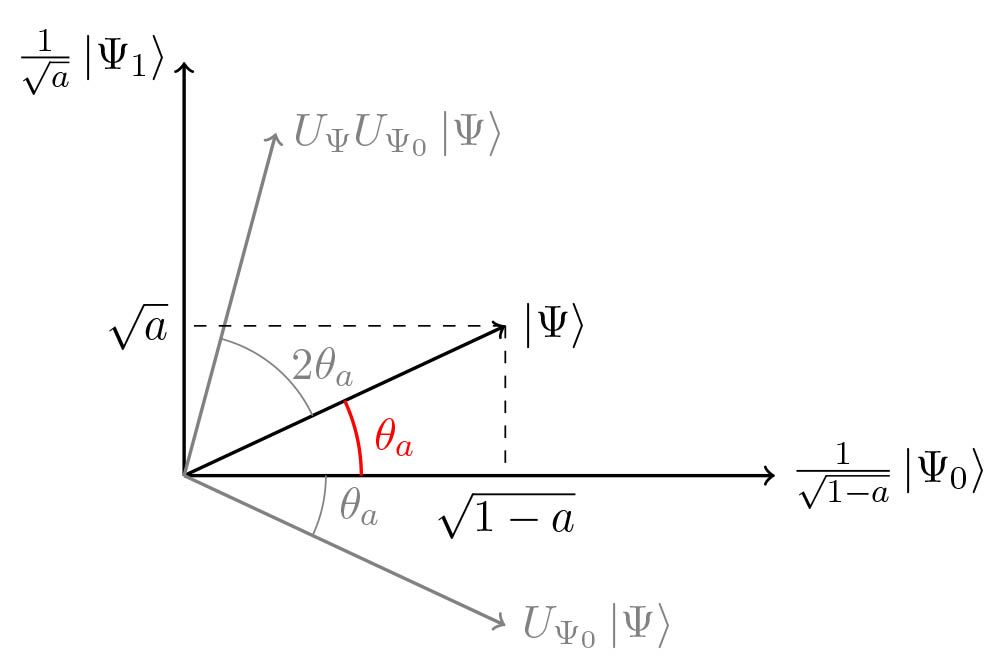
\[\begin{aligned} Q\left\vert \Psi_{1}\right\rangle &=U_{\Psi} U_{\Psi_{0}}\left\vert \Psi_{1}\right\rangle=-U_{\Psi}\left\vert \Psi_{1}\right\rangle=(I-2\vert \Psi\rangle\langle\Psi\vert )\left\vert \Psi_{1}\right\rangle \\ &=\left\vert \Psi_{1}\right\rangle-2 a\vert \Psi\rangle=(1-2 a)\left\vert \Psi_{1}\right\rangle-2 a\left\vert \Psi_{0}\right\rangle \\ Q\left\vert \Psi_{0}\right\rangle &=U_{\Psi}\left\vert \Psi_{0}\right\rangle=(2\vert \Psi\rangle\langle\Psi\vert -I)\left\vert \Psi_{0}\right\rangle \\ &=2(1-a)\vert \Psi\rangle-\left\vert \Psi_{0}\right\rangle=2(1-a)\left\vert \Psi_{1}\right\rangle+(1-2 a)\left\vert \Psi_{0}\right\rangle \end{aligned}\]Using \(\sin ^{2}\left(\theta_{a}\right)=a\) and \(\cos ^{2}\left(\theta_{a}\right)=1-a\), we get:
\[\begin{aligned} Q \frac{\left\vert \Psi_{1}\right\rangle}{\sqrt{a}} &=(1-2 a) \frac{\left\vert \Psi_{1}\right\rangle}{\sqrt{a}}-2 \sqrt{a(1-a)} \frac{\left\vert \Psi_{0}\right\rangle}{\sqrt{1-a}} \\ &=\left(1-2 \sin ^{2}\left(\theta_{a}\right)\right) \frac{\left\vert \Psi_{1}\right\rangle}{\sqrt{a}}-2 \cos \left(\theta_{a}\right) \sin \left(\theta_{a}\right) \frac{\left\vert \Psi_{0}\right\rangle}{\sqrt{1-a}} \\ &=\cos \left(2 \theta_{a}\right) \frac{\left\vert \Psi_{1}\right\rangle}{\sqrt{a}}-\sin \left(2 \theta_{a}\right) \frac{\left\vert \Psi_{0}\right\rangle}{\sqrt{1-a}} \\ Q \frac{\left\vert \Psi_{0}\right\rangle}{\sqrt{1-a}} &=\sin \left(2 \theta_{a}\right) \frac{\left\vert \Psi_{1}\right\rangle}{\sqrt{a}}+\cos \left(2 \theta_{a}\right) \frac{\left\vert \Psi_{0}\right\rangle}{\sqrt{1-a}} \end{aligned}\]Thus, \(Q\) is a rotation matrix in the basis \(\frac{1}{\sqrt{a}}\left\vert \Psi_{1}\right\rangle, \frac{1}{\sqrt{1-a}}\left\vert \Psi_{0}\right\rangle\)
\[Q=\left(\begin{array}{cc} \cos 2 \theta_{a} & \sin 2 \theta_{a} \\ -\sin 2 \theta_{a} & \cos 2 \theta_{a} \end{array}\right)\]It has eigenvalues \(e^{2 i \theta_{a}}, e^{-2 i \theta_{a}}\) with corresponding eigenvectors \(\frac{1}{2}(1 i), \frac{1}{2}(1-i)\), noted
\[\left\vert \Psi_{+}\right\rangle\]and
\(\left\vert \Psi_{-}\right\rangle\) .
We can now write \(\vert \Psi\rangle\) in the \(Q\)-eigenvector basis:
\[\vert \Psi\rangle=\frac{-i}{2}\left(e^{i \theta_{a}}\left\vert \Psi_{+}\right\rangle-e^{-i \theta_{a}}\left\vert \Psi_{-}\right\rangle\right)\]and it follows that: \(Q^{j}\vert \Psi\rangle=\frac{-i}{2}\left(e^{(2 j+1) i \theta_{a}}\left\vert \Psi_{+}\right\rangle-e^{-(2 j+1) i \theta_{a}}\left\vert \Psi_{-}\right\rangle\right)\)
By writing it back in the original \(\frac{1}{\sqrt{a}}\left\vert \Psi_{1}\right\rangle, \frac{1}{\sqrt{1-a}}\left\vert \Psi_{0}\right\rangle\) basis: \(Q^{j}\vert \Psi\rangle=\sin \left((2 j+1) \theta_{a}\right) \frac{1}{\sqrt{a}}\left\vert \Psi_{1}\right\rangle+\cos \left((2 j+1) \theta_{a}\right) \frac{1}{\sqrt{1-a}}\left\vert \Psi_{0}\right\rangle\)
2. How to speed up the process by circuit design?
The basic idea is that we can levarage Quantum Amplititude Estimation to achieve a quadratic speedup since the information we want are included in the amplititutde.
AE uses \(m\) additional sampling qubits and Quantum Phase Estimation to produce an estimator \(\)\tilde{a}=\sin ^{2}(y \pi / M)\(of\)a\(, where\) \(y \in\{0, \ldots, M-1\}\) and \(M\) (the number of samples, is \(2^{m}\)). The estimator \(\tilde{a}\) satisfies
\[\vert a-\tilde{a}\vert \leq \frac{\pi}{M}+\frac{\pi^{2}}{M^{2}}=O\left(M^{-1}\right) \text {, }\]with probability of at least \(8 / \pi^{2}\). This represents a quadratic speedup compared to the \(O\left(M^{-1 / 2}\right)\) convergence rate of classical Monte Carlo methods.
Q: how we can result a quadratic speedup?
A: M is the number of samples, with accraucy \(\epsilon\), classical monte carlo simulation needs t times repetation, just like t times of sampling.
\[t=\mathcal{O}\left(\frac{\mu(1-\mu)}{\epsilon^{2}}\right)\]Quantum Monte Carlo Simulation needs evaluations of function f: \(M=\mathcal{O}\left(\frac{1}{\epsilon \sqrt{\mu}}\right)\)
Q: How can we interpret the M in amplititude estimation? M should be the evalutions of function f, but I also read some ideas that say it it also the number of reflections during the algorithm.
Overall, we can see the task of the quantum algorithm will be to improve the \(\epsilon\) dependence from \(\epsilon^{2}\) to \(\epsilon\).
To use \(A E\) to estimate quantities related to a random variable \(X\) we must first represent \(X\) as a quantum state. Using \(n\) qubits we \(\operatorname{map} X\) to the interval \(\{0, \ldots, N-1\}\), where \(N=2^{n} . X\) is then represented by the state
\[\mathcal{R}\vert 0\rangle_{n}=\vert \psi\rangle_{n}=\sum_{i=0}^{N-1} \sqrt{p_{i}}\vert i\rangle_{n} \quad \text { with } \sum_{i=0}^{N-1} p_{i}=1\]We now look at the overall circuit for this problem.

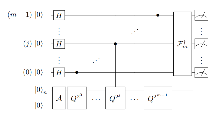
For phase estimation, we require the conditional application of the operation \(\mathcal{Q}\). Concretely, we require \(\mathcal{Q}^{c}:\vert j\rangle\vert \psi\rangle \rightarrow\vert j\rangle \mathcal{Q}^{j}\vert \psi\rangle\)
for an arbitrary \(n\) qubit state \(\vert \psi\rangle\) . Phase estimation then proceeds in the following way, see Fig. 2 (c). Take a copy of \(\vert \chi\rangle\)
by applying \(\mathcal{F}\) to a register of qubits in \(\left\vert 0^{n+1}\right\rangle\) . Then prepare an additional \(m\)-qubit register in the uniform superposition via the Hadamard operation \(\mathcal{H}\)
\[\mathcal{H}^{\otimes m}\left\vert 0^{m}\right\rangle\vert \chi\rangle=\frac{1}{\sqrt{2^{m}}} \sum_{j=0}^{2^{m}-1}\vert j\rangle\vert \chi\rangle\]Then perform the controlled operation \(\mathcal{Q}^{c}\) to obtain
\[\frac{1}{\sqrt{2^{m}}} \sum_{j=0}^{2^{m}-1}\vert j\rangle \mathcal{Q}^{j}\vert \chi\rangle\]One can show that \(\vert \chi\rangle=\frac{1}{\sqrt{2}}\left(\left\vert \psi_{+}\right\rangle+\left\vert \psi_{-}\right\rangle\right)\) is the expansion of \(\vert \chi\rangle\) into the two eigenvectors of \(\mathcal{Q}\) corresponding to the eigenvalues \(e^{\pm i \theta}\) . An inverse quantum Fourier transformation applied to prepare the state
\[\sum_{x=0}^{2^{m}-1} \alpha_{+}(x)\vert x\rangle\left\vert \psi_{+}\right\rangle+\alpha_{-}(x)\vert x\rangle\left\vert \psi_{-}\right\rangle\]The \(\left\vert \alpha_{\pm}(x)\right\vert ^{2}\) are peaked where \(x / 2^{m}=\pm \hat{\theta}\) is an \(m\)-bit approximation to \(\pm \theta\) . Hence, measurement of the \(\vert x\rangle\) register will retrieve the approximations \(\pm \hat{\theta}\) .
Overall, quantum amplititude estimation can help us to find \(\tilde{a}=\sin ^{2}(y \pi / M)\)
Maximum Likelihood Estimation
There are many methods for estimating unknown parameters from data. We will first consider the maximum likelihood estimate (MLE), which answers the question:
- For which parameter value does the observed data have the biggest probability?
The MLE is an example of a point estimate because it gives a single value for the unknown parameter (later our estimates will involve intervals and probabilities). Two advantages of the MLE are that it is often easy to compute and that it agrees with our intuition in simple examples. We will explain the MLE through a series of examples.
Example A coin is flipped 100 times. Given that there were 55 heads, find the maximum likelihood estimate for the probability \(p\) of heads on a single toss. Before actually solving the problem, let’s establish some notation and terms. We can think of counting the number of heads in 100 tosses as an experiment. For a given value of \(p\), the probability of getting 55 heads in this experiment is the binomial probability \(P(55 \text { heads })=\left(\begin{array}{c} 100 \\ 55 \end{array}\right) p^{55}(1-p)^{45}\) The probability of getting 55 heads depends on the value of \(p\), so let’s include \(p\) in by using the notation of conditional probability: \(P(55 \text { heads } \mid p)=\left(\begin{array}{c} 100 \\ 55 \end{array}\right) p^{55}(1-p)^{45}\) You should read \(P(55 heads \mid p)\) as: ‘the probability of 55 heads given \(p\),’ or more precisely as ‘the probability of 55 heads given that the probability of heads on a single toss is \(p\)
Here are some standard terms we will use as we do statistics.
- Experiment: Flip the coin 100 times and count the number of heads.
- Data: The data is the result of the experiment. In this case it is ‘ 55 heads’.
- Parameter(s) of interest: We are interested in the value of the unknown parameter \(p\)
- Likelihood, or likelihood function: this is \(P( data \mid p)\) . Note it is a function of both the data and the parameter \(p\). In this case the likelihood is \(P(55 \text { heads } \mid p)=\left(\begin{array}{c} 100 \\ 55 \end{array}\right) p^{55}(1-p)^{45}\)
Definition: Given data the maximum likelihood estimate (MLE) for the parameter \(p\) is the value of \(p\) that maximizes the likelihood \(P(data \mid p)\) . That is, the MLE is the value of \(p\) for which the data is most likely. answer: For the problem at hand, we saw above that the likelihood \(P(55 \text { heads } \mid p)=\left(\begin{array}{c} 100 \\ 55\end{array}\right) p^{55}(1-p)^{45}\) We’ll use the notation \(\hat{p}\) for the MLE. We use calculus to find it by taking the derivative of the likelihood function and setting it to 0 . \(\frac{d}{d p} P(\text { data } \mid p)=\left(\begin{array}{c} 100 \\ 55 \end{array}\right)\left(55 p^{54}(1-p)^{45}-45 p^{55}(1-p)^{44}\right)=0\) Solving this for \(p\) we get \(\begin{aligned} &55 p^{54}(1-p)^{45}=45 p^{55}(1-p)^{44} \\ &55(1-p)=45 p \\ &55=100 p \end{aligned}\) the MLE is \(\hat{p}=.55\) Note:
- The MLE for \(p\) turned out to be exactly the fraction of heads we saw in our data.
- The MLE is computed from the data. That is, it is a statistic.
- Officially you should check that the critical point is indeed a maximum. You can do this with the second derivative test.
QAE + MLE

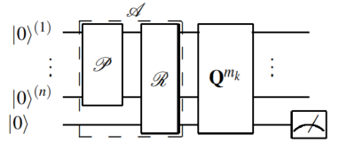
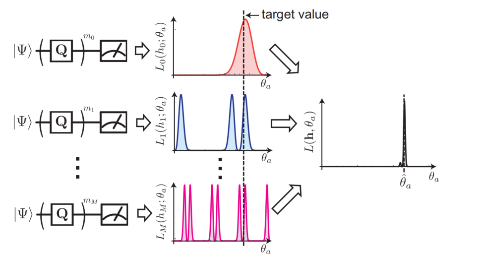
The idea of QAE + MLE is to use quantum amplification to amplify angle \(\theta\). And measure the result of the objective state. For example, in the above figure, we can get one result for each shot. And then we can measure several times can get lots of 0 and 1 (good result).
Then we solve the parameter \(\theta\) with Maximum Likelihood Estimation.

Code
import matplotlib.pyplot as plt

%matplotlib inline
import numpy as np

from qiskit import Aer, QuantumCircuit
from qiskit.utils import QuantumInstance
from qiskit.algorithms import IterativeAmplitudeEstimation, EstimationProblem
from qiskit.circuit.library import LinearAmplitudeFunction
from qiskit.circuit.library import LogNormalDistribution, LinearAmplitudeFunction

from typing import Optional, List, Union, Tuple, Dict, Callable
import numpy as np
from scipy.optimize import brute
from scipy.stats import norm, chi2

from qiskit.providers import BaseBackend
from qiskit.providers import Backend
from qiskit import ClassicalRegister, QuantumRegister, QuantumCircuit
from qiskit.utils import QuantumInstance

from qiskit.algorithms import AmplitudeEstimator, AmplitudeEstimatorResult
from qiskit.algorithms import EstimationProblem
from qiskit.algorithms import AlgorithmError

"""The Maximum Likelihood Amplitude Estimation algorithm."""

MINIMIZER = Callable[[Callable[[float], float], List[Tuple[float, float]]], float]

class MaximumLikelihoodAmplitudeEstimation(AmplitudeEstimator):
    def __init__(
        self,
        evaluation_schedule: Union[List[int], int],
        minimizer: Optional[MINIMIZER] = None,
        quantum_instance: Optional[Union[QuantumInstance, BaseBackend, Backend]] = None,
    ) -> None:
        r"""
        Args:
            evaluation_schedule: If a list, the powers applied to the Grover operator. The list
                element must be non-negative. If a non-negative integer, an exponential schedule is
                used where the highest power is 2 to the integer minus 1:
                `[id, Q^2^0, ..., Q^2^(evaluation_schedule-1)]`.
            minimizer: A minimizer used to find the minimum of the likelihood function.
                Defaults to a brute search where the number of evaluation points is determined
                according to ``evaluation_schedule``. The minimizer takes a function as first
                argument and a list of (float, float) tuples (as bounds) as second argument and
                returns a single float which is the found minimum.
            quantum_instance: Quantum Instance or Backend

        Raises:
            ValueError: If the number of oracle circuits is smaller than 1.
        """

        super().__init__()

        # set quantum instance
        self.quantum_instance = quantum_instance

        # get parameters
        if isinstance(evaluation_schedule, int):
            if evaluation_schedule < 0:
                raise ValueError("The evaluation schedule cannot be < 0.")
            print([0] + [2 ** j for j in range(evaluation_schedule)])
            self._evaluation_schedule = [0] + [2 ** j for j in range(evaluation_schedule)]
        else:
            if any(value < 0 for value in evaluation_schedule):
                raise ValueError("The elements of the evaluation schedule cannot be < 0.")

            self._evaluation_schedule = evaluation_schedule

        if minimizer is None:
            # default number of evaluations is max(10^4, pi/2 * 10^3 * 2^(m))
            nevals = max(10000, int(np.pi / 2 * 1000 * 2 * self._evaluation_schedule[-1]))

            def default_minimizer(objective_fn, bounds):
                return brute(objective_fn, bounds, Ns=nevals)[0]

            self._minimizer = default_minimizer
        else:
            self._minimizer = minimizer

    @property
    def quantum_instance(self) -> Optional[QuantumInstance]:
        """Get the quantum instance.

        Returns:
            The quantum instance used to run this algorithm.
        """
        return self._quantum_instance

    @quantum_instance.setter
    def quantum_instance(
        self, quantum_instance: Union[QuantumInstance, BaseBackend, Backend]
    ) -> None:
        """Set quantum instance.

        Args:
            quantum_instance: The quantum instance used to run this algorithm.
        """
        if isinstance(quantum_instance, (BaseBackend, Backend)):
            quantum_instance = QuantumInstance(quantum_instance)
        self._quantum_instance = quantum_instance

    def construct_circuits(
        self, estimation_problem: EstimationProblem, measurement: bool = False
    ) -> List[QuantumCircuit]:
        """Construct the Amplitude Estimation w/o QPE quantum circuits.
        Args:
            estimation_problem: The estimation problem for which to construct the QAE circuit.
            measurement: Boolean flag to indicate if measurement should be included in the circuits.
        Returns:
            A list with the QuantumCircuit objects for the algorithm.
        """
        # keep track of the Q-oracle queries
        circuits = []

        num_qubits = max(
            estimation_problem.state_preparation.num_qubits,
            estimation_problem.grover_operator.num_qubits,
        )
        $$
        q = QuantumRegister(num_qubits, "q")
        qc_0 = QuantumCircuit(q, name="qc_a")

        # add classical register if needed
        if measurement:
            c = ClassicalRegister(len(estimation_problem.objective_qubits))
            qc_0.add_register(c)

        # add two circuits
        qc_0.compose(estimation_problem.state_preparation, inplace=True)

        for k in self._evaluation_schedule:
            qc_k = qc_0.copy(name="qc_a_q_%s" % k)
            $$
            if k != 0:
                qc_k.compose(estimation_problem.grover_operator.power(k), inplace=True)

            if measurement:
                # real hardware can currently not handle operations after measurements,
                # which might happen if the circuit gets transpiled, hence we're adding
                # a safeguard-barrier
                qc_k.barrier()
                qc_k.measure(estimation_problem.objective_qubits, c[:])

            circuits += [qc_k]
            print("j:", k)
            print(qc_k.draw())
        $$
        return circuits

    $$
    def compute_mle(
        self,
        circuit_results: Union[List[Dict[str, int]], List[np.ndarray]],
        estimation_problem: EstimationProblem,
        num_state_qubits: Optional[int] = None,
        return_counts: bool = False,
    ) -> Union[float, Tuple[float, List[float]]]:
        """Compute the MLE via a grid-search.

        This is a stable approach if sufficient gridpoints are used.

        Args:
            circuit_results: A list of circuit outcomes. Can be counts or statevectors.
            estimation_problem: The estimation problem containing the evaluation schedule and the
                number of likelihood function evaluations used to find the minimum.
            num_state_qubits: The number of state qubits, required for statevector simulations.
            return_counts: If True, returns the good counts.

        Returns:
            The MLE for the provided result object.
        """
        good_counts, all_counts = _get_counts(circuit_results, estimation_problem, num_state_qubits)

        # search range
        eps = 1e-15  # to avoid invalid value in log
        search_range = [0 + eps, np.pi / 2 - eps]

        def loglikelihood(theta):
            # loglik contains the first `it` terms of the full loglikelihood
            loglik = 0
            for i, k in enumerate(self._evaluation_schedule):
                angle = (2 * k + 1) * theta
                loglik += np.log(np.sin(angle) ** 2) * good_counts[i]
                loglik += np.log(np.cos(angle) ** 2) * (all_counts[i] - good_counts[i])
            return -loglik
        $$
        est_theta = self._minimizer(loglikelihood, [search_range])

        if return_counts:
            return est_theta, good_counts
        return est_theta

    def estimate(
        self, estimation_problem: EstimationProblem
    ) -> "MaximumLikelihoodAmplitudeEstimationResult":
        if estimation_problem.state_preparation is None:
            raise AlgorithmError(
                "Either the state_preparation variable or the a_factory "
                "(deprecated) must be set to run the algorithm."
            )

        result = MaximumLikelihoodAmplitudeEstimationResult()
        result.evaluation_schedule = self._evaluation_schedule
        result.minimizer = self._minimizer
        result.post_processing = estimation_problem.post_processing

        if self._quantum_instance.is_statevector:
            # run circuit on statevector simulator
            circuits = self.construct_circuits(estimation_problem, measurement=False)
            ret = self._quantum_instance.execute(circuits)

            # get statevectors and construct MLE input
            statevectors = [np.asarray(ret.get_statevector(circuit)) for circuit in circuits]
            result.circuit_results = statevectors

            # to count the number of Q-oracle calls (don't count shots)
            result.shots = 1

        else:
            # run circuit on QASM simulator
            circuits = self.construct_circuits(estimation_problem, measurement=True)
            ret = self._quantum_instance.execute(circuits)

            # get counts and construct MLE input
            result.circuit_results = [ret.get_counts(circuit) for circuit in circuits]

            # to count the number of Q-oracle calls
            result.shots = self._quantum_instance._run_config.shots

        # run maximum likelihood estimation
        num_state_qubits = circuits[0].num_qubits - circuits[0].num_ancillas
        theta, good_counts = self.compute_mle(
            result.circuit_results, estimation_problem, num_state_qubits, True
        )
        $$
        # store results
        result.theta = theta
        result.good_counts = good_counts
        result.estimation = np.sin(result.theta) ** 2

        return result


class MaximumLikelihoodAmplitudeEstimationResult(AmplitudeEstimatorResult):
    """The ``MaximumLikelihoodAmplitudeEstimation`` result object."""

    def __init__(self) -> None:
        super().__init__()
        self._theta = None
        self._minimizer = None
        self._good_counts = None
        self._evaluation_schedule = None
        self._fisher_information = None

    @property
    def theta(self) -> float:
        r"""Return the estimate for the angle :math:`\theta`."""
        return self._theta

    @theta.setter
    def theta(self, value: float) -> None:
        r"""Set the estimate for the angle :math:`\theta`."""
        self._theta = value

    @property
    def minimizer(self) -> callable:
        """Return the minimizer used for the search of the likelihood function."""
        return self._minimizer

    @minimizer.setter
    def minimizer(self, value: callable) -> None:
        """Set the number minimizer used for the search of the likelihood function."""
        self._minimizer = value

    @property
    def good_counts(self) -> List[float]:
        """Return the percentage of good counts per circuit power."""
        return self._good_counts

    @good_counts.setter
    def good_counts(self, counts: List[float]) -> None:
        """Set the percentage of good counts per circuit power."""
        self._good_counts = counts

    @property
    def evaluation_schedule(self) -> List[int]:
        """Return the evaluation schedule for the powers of the Grover operator."""
        return self._evaluation_schedule

    @evaluation_schedule.setter
    def evaluation_schedule(self, evaluation_schedule: List[int]) -> None:
        """Set the evaluation schedule for the powers of the Grover operator."""
        self._evaluation_schedule = evaluation_schedule


def _get_counts(
    circuit_results: List[Union[np.ndarray, List[float], Dict[str, int]]],
    estimation_problem: EstimationProblem,
    num_state_qubits: int,
) -> Tuple[List[float], List[int]]:
    """Get the good and total counts.

    Returns:
        A pair of two lists, ([1-counts per experiment], [shots per experiment]).

    Raises:
        AlgorithmError: If self.run() has not been called yet.
    """
    one_hits = []  # h_k: how often 1 has been measured, for a power Q^(m_k)
    all_hits = []  # shots_k: how often has been measured at a power Q^(m_k)
    if all(isinstance(data, (list, np.ndarray)) for data in circuit_results):
        probabilities = []
        num_qubits = int(np.log2(len(circuit_results[0])))  # the total number of qubits
        for statevector in circuit_results:
            p_k = 0.0
            for i, amplitude in enumerate(statevector):
                probability = np.abs(amplitude) ** 2
                # consider only state qubits and revert bit order
                bitstr = bin(i)[2:].zfill(num_qubits)[-num_state_qubits:][::-1]
                objectives = [bitstr[index] for index in estimation_problem.objective_qubits]
                if estimation_problem.is_good_state(objectives):
                    p_k += probability
            probabilities += [p_k]

        one_hits = probabilities
        all_hits = np.ones_like(one_hits)
    else:
        for counts in circuit_results:
            all_hits.append(sum(counts.values()))
            one_hits.append(
                sum(
                    count
                    for bitstr, count in counts.items()
                    if estimation_problem.is_good_state(bitstr)
                )
            )
    $$
    print("one_hits", one_hits)
    print("all_hits", all_hits)
    return one_hits, all_hits
Expectation Computing
We can implement a rotation onto an ancilla qubit that we can input information into circuit:
\[\mathcal{R}\vert x\rangle\vert 0\rangle=\vert x\rangle(\sqrt{1-v(x)}\vert 0\rangle+\sqrt{v(x)}\vert 1\rangle)\]In this equation, \(v\) could be the price of assets and some other information.
\(A\) is an algorithm to describe the distribution of \(x\).
\(v(A)\) denotes the random variable specified by the algorithm \(A\) and the function \(v(x)\).
\[\mathbb{E}[v(\mathcal{A})]:=\sum_{x=0}^{2^{n}-1}\left\vert a_{x}\right\vert ^{2} v(x)\]- Apply the algorithm \(A\),
where \(\left\vert 0^{n}\right\rangle\) denotes the \(n\) qubit register with all qubits in the state \(\vert 0\rangle\).
- Perform the rotation of an ancilla via \(\mathcal{R}\): \(\begin{gathered} \sum_{x=0}^{2^{n}-1} a_{x}\vert x\rangle\vert 0\rangle \\ \rightarrow \sum_{x=0}^{2^{n}-1} a_{x}\vert x\rangle(\sqrt{1-v(x)}\vert 0\rangle+\sqrt{v(x)}\vert 1\rangle)=:\vert \chi\rangle \end{gathered}\)
- Measure the ancilla in the state \(\vert 1 \rangle\) obtains as the success probability of the expectation value \(\mu:=\left\langle\chi\left\vert \left(\mathcal{I}_{2^{n}} \otimes\vert 1\rangle\langle 1\vert \right)\right\vert \chi\right\rangle=\sum_{x=0}^{2^{n}-1}\left\vert a_{x}\right\vert ^{2} v(x) \equiv \mathbb{E}[v(\mathcal{A})]\) .
This success probability can be obtained by repeating the procedure \(t\) times and collecting the clicks for the \(\vert 1 \rangle\) state as a fraction of the total measurements. The variance is \(\epsilon^{2}=\frac{\mu(1-\mu)}{t}\) from the Bernoulli distribution, i.e. the standard deviation is \(\epsilon=\sqrt{\frac{\mu(1-\mu)}{t}}\) . Hence, the experiment has to be repeated \(t=\mathcal{O}\left(\frac{\mu(1-\mu)}{\epsilon^{2}}\right)\)
Note that we can slightly redefine the quantity being measured. Define the unitary
\[\mathcal{V}:=\mathcal{I}_{2^{n+1}}-2 \mathcal{I}_{2^{n}} \otimes\vert 1\rangle\langle 1\vert ,\]for which \(\mathcal{V}=\mathcal{V}^{\dagger}\) and \(\mathcal{V}^{2}=\mathcal{I}_{2^{n+1}} .\) A measurement of \(\mathcal{V}\) on \(\vert \chi\rangle\) obtains \(\langle\chi\vert \mathcal{V}\vert \chi\rangle=1-2 \mu\)
From this measurement we can extract the desired expectation value. Any quantum state in the \((n+1)\)-qubit Hilbert space can be expressed as a linear combination of \(\vert \chi\rangle\) and a specific orthogonal complement \(\left\vert \chi^{\perp}\right\rangle\)
Thus, we can express \(\mathcal{V}\vert \chi\rangle=\cos (\theta / 2)\vert \chi\rangle+e^{i \phi} \sin (\theta / 2)\left\vert \chi^{\perp}\right\rangle\) , with the angles \(\phi\) and \(\theta\) . Note that our expectation value can be retrieved via
\[1-2 \mu=\cos (\theta / 2)\]The task becomes to measure \(\theta\)
This quadratic dependency is analogous to the classical Monte Carlo dependency.
Option Pricing
3. How can we use this technique to price options?
We need to design a function that encode the expected value into the \(sin\) function.
Taking a dffierent step, we can set \(f(i)\) inside sin function \(sin(f(i))\).
The payoff function for the option contracts of interest is piece-wise linear and as such we only need to consider linear functions \(f:\left\{0, \ldots, 2^{n}-1\right\} \rightarrow[0,1]\) which we write \(f(i)=f_{1} i+f_{0}\)
We can efficiently create an operator that performs \(\vert i\rangle_{n}\vert 0\rangle \rightarrow\vert i\rangle_{n}(\cos [f(i)]\vert 0\rangle+\sin [f(i)]\vert 1\rangle)\)
using controlled Y-rotations.
We now describe how to obtain \(\mathbb{E}[f(X)]\) for a linear function \(f\) of a random variable \(X\) which is mapped to integer values \(i \in\left\{0, \ldots, 2^{n}-1\right\}\)
that occur with probability \(p_{i}\) respectively. To do this we use the procedure outlined immediately above to create the operator that maps \(\sum_{i} \sqrt{p_{i}}\vert i\rangle_{n}\vert 0\rangle\)
to
\[\sum_{i=0}^{2^{n}-1} \sqrt{p_{i}}\vert i\rangle_{n}\left[\cos \left(c \tilde{f}(i)+\frac{\pi}{4}\right)\vert 0\rangle+\sin \left(c \tilde{f}(i)+\frac{\pi}{4}\right)\vert 1\rangle\right]\]where \(\tilde{f}(i)\) is a scaled version of \(f(i)\) given by
\[\tilde{f}(i)=2 \frac{f(i)-f_{\min }}{f_{\max }-f_{\min }}-1,\]with \(f_{\min }=\min _{i} f(i)\)
and \(f_{\max }=\max _{i} f(i)\)
and \(c \in[0,1]\) is an additional scaling parameter. The relation is chosen so that \(\tilde{f}(i) \in[-1,1]\)
Consequently,
\(\sin ^{2}[c \tilde{f}(i)+\pi / 4]\) is an anti-symmetric function around \(\tilde{f}(i)=0\) With these definitions, the probability to find the ancilla qubit in state
\(\vert 1\rangle\) , namely
\[P_{1}=\sum_{i=0}^{2^{n}-1} p_{i} \sin ^{2}\left(c \tilde{f}(i)+\frac{\pi}{4}\right)\]is well approximated by
\[P_{1} \approx \sum_{i=0}^{2^{n}-1} p_{i}\left(c \tilde{f}(i)+\frac{1}{2}\right)=c \frac{2 \mathbb{E}[f(X)]-f_{\min }}{f_{\max }-f_{\min }}-c+\frac{1}{2} .\]To obtain this result we made use of the approximation
\[\sin ^{2}\left(c \tilde{f}(i)+\frac{\pi}{4}\right)=c \tilde{f}(i)+\frac{1}{2}+\mathcal{O}\left(c^{3} \tilde{f}^{3}(i)\right)\]which is valid for small values of \(c \tilde{f}(i)\) .
Therefore, by evaluating \(\sin ^{2}\left(c \tilde{f}(i)+\frac{\pi}{4}\right)\) we can find \(\tilde{f}(i)\) easily and to know the \(\mathbb{E}[f(X)]\).
 # number of qubits to represent the uncertainty
num_uncertainty_qubits = 3

# parameters for considered random distribution
S = 2.0  # initial spot price
vol = 0.1  # volatility of 40%
r = 0.04  # annual interest rate of 4%
T = 300 / 365  # 40 days to maturity

# resulting parameters for log-normal distribution
mu = (r - 0.5 * vol ** 2) * T + np.log(S)
sigma = vol * np.sqrt(T)
mean = np.exp(mu + sigma ** 2 / 2)
variance = (np.exp(sigma ** 2) - 1) * np.exp(2 * mu + sigma ** 2)
stddev = np.sqrt(variance)

# lowest and highest value considered for the spot price; in between, an equidistant discretization is considered.
low = np.maximum(0, mean - 3 * stddev)
high = mean + 3 * stddev

# construct A operator for QAE for the payoff function by
# composing the uncertainty model and the objective
uncertainty_model = LogNormalDistribution(
    num_uncertainty_qubits, mu=mu, sigma=sigma ** 2, bounds=(low, high)
)
 $$

 # plot probability distribution
x = uncertainty_model.values
y = uncertainty_model.probabilities
plt.bar(x, y, width=0.2)
plt.xticks(x, size=15, rotation=90)
plt.yticks(size=15)
plt.grid()
plt.xlabel("Spot Price at Maturity $$S_T$$ (\$$)", size=15)
plt.ylabel("Probability ($$\%$$)", size=15)
plt.show()

# set the strike price (should be within the low and the high value of the uncertainty)
strike_price = 2

# set the approximation scaling for the payoff function
c_approx = 0.1

# setup piecewise linear objective fcuntion
breakpoints = [low, strike_price]
slopes = [0, 1]
offsets = [0, 0]
f_min = 0
f_max = high - strike_price
european_call_objective = LinearAmplitudeFunction(
    num_uncertainty_qubits,
    slopes,
    offsets,
    domain=(low, high),
    image=(f_min, f_max),
    breakpoints=breakpoints,
    rescaling_factor=c_approx,
)

# construct A operator for QAE for the payoff function by
# composing the uncertainty model and the objective
num_qubits = european_call_objective.num_qubits
european_call = QuantumCircuit(num_qubits)
european_call.append(uncertainty_model, range(num_uncertainty_qubits))
european_call.append(european_call_objective, range(num_qubits))

# draw the circuit
european_call.draw()

from qiskit import BasicAer
from qiskit.utils import QuantumInstance

problem = EstimationProblem(
    state_preparation=european_call,
    objective_qubits=[3]
)

backend = BasicAer.get_backend("statevector_simulator")
quantum_instance = QuantumInstance(backend)

# construct amplitude estimation
ae = MaximumLikelihoodAmplitudeEstimation(
    evaluation_schedule=4,
    quantum_instance=quantum_instance)
result = ae.estimate(problem)

european_call_objective.post_processing(result.estimation)
Experiment Reproducement for JP Morgan’s paper Stamatopoulos, Nikitas, et al. "Option pricing using quantum computers." Quantum 4 (2020): 291.
Reference:
1. Nielsen, Michael A., and Isaac Chuang. "Quantum computation and quantum information." (2002): 558-559.
2. Asfaw, Abraham, et al. "Learn quantum computation using qiskit." Accessed: Oct 24 (2020): 2020.
3. Susskind, Leonard, and Art Friedman. Quantum mechanics: the theoretical minimum. Basic Books, 2014.
4. Rebentrost, Patrick; Gupt, Brajesh; Bromley, Thomas R. (2018): Quantum computational finance: Monte Carlo pricing of financial derivatives. In Phys. Rev. A 98 (2), p. 41. DOI: 10.1103/PhysRevA.98.022321.
5. Brassard, Gilles, et al. "Quantum amplitude amplification and estimation." Contemporary Mathematics 305 (2002): 53-74.
6. Stamatopoulos, Nikitas, et al. "Option pricing using quantum computers." Quantum 4 (2020): 291.
7. Y. Suzuki, S. Uno, R. Raymond, T. Tanaka, T. Onodera, and N. Yamamoto, “Amplitude estimation without phase estimation,” Quantum Inf Process, vol. 19, no. 2, p. 75, Feb. 2020, doi: 10.1007/s11128-019-2565-2.