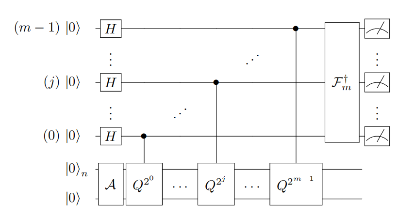
For the pricing problem in finance, the main challenge is to compute an expectation value of a function of one or more underlying stochastic financial assets. For models beyond BSM, such pricing is often performed via Monte Carlo evaluation. Quantum Monte Carlo simulation would have a quadratic speedup compared to classical one.
1. How quantum computing can result an expectation value?
We can implement a rotation onto an ancilla qubit that we can input information into circuit:
\[\mathcal{R}\vert x\rangle\vert 0\rangle=\vert x\rangle(\sqrt{1-v(x)}\vert 0\rangle+\sqrt{v(x)}\vert 1\rangle)\]In this equation, \(v\) could be the price of assets and some other information.
Then we can mesaure \(\mathbb{E}[v(\mathcal{A})]\)
\(A\) is an algorithm to describe the distribution of \(x\).
\(v(A)\) denotes the random variable specified by the algorithm \(A\) and the function \(v(x)\).
\[\mathbb{E}[v(\mathcal{A})]:=\sum_{x=0}^{2^{n}-1}\left\vert a_{x}\right\vert ^{2} v(x)\]-
Apply the algorithm \(A\),
\[\mathcal{A}\left\vert 0^{n}\right\rangle=\sum_{x=0}^{2^{n}-1} a_{x}\vert x\rangle\]where \(\left\vert 0^{n}\right\rangle\) denotes the \(n\) qubit register with all qubits in the state \(\vert 0\rangle\).
- Perform the rotation of an ancilla via \(\mathcal{R}\) \(\begin{gathered} \sum_{x=0}^{2^{n}-1} a_{x}\vert x\rangle\vert 0\rangle \\ \rightarrow \sum_{x=0}^{2^{n}-1} a_{x}\vert x\rangle(\sqrt{1-v(x)}\vert 0\rangle+\sqrt{v(x)}\vert 1\rangle)=:\vert \chi\rangle \end{gathered}\)
- Measure the ancilla in the state \(\vert 1 \rangle\) obtains as the success probability of the expectation value \(\mu:=\left\langle\chi\left\vert \left(\mathcal{I}_{2^{n}} \otimes\vert 1\rangle\langle 1\vert \right)\right\vert \chi\right\rangle=\sum_{x=0}^{2^{n}-1}\left\vert a_{x}\right\vert ^{2} v(x) \equiv \mathbb{E}[v(\mathcal{A})] .\)
This success probability can be obtained by repeating the procedure \(t\) times and collecting the clicks for the \(\vert 1 \rangle\) state as a fraction of the total measurements. The variance is \(\epsilon^{2}=\frac{\mu(1-\mu)}{t}\) from the Bernoulli distribution, i.e. the standard deviation is \(\epsilon=\sqrt{\frac{\mu(1-\mu)}{t}}\). Hence, the experiment has to be repeated \(t=\mathcal{O}\left(\frac{\mu(1-\mu)}{\epsilon^{2}}\right)\)
This quadratic dependency is analogous to the classical Monte Carlo dependency.
2. How to speed up the process by circuit design?
The basic idea is that we can levarage Quantum Amplititude Estimation to achieve a quadratic speedup since the information we want are included in the amplititutde.
AE Estimation Review
AE uses \(m\) additional sampling qubits and Quantum Phase Estimation to produce an estimator \(\tilde{a}=\sin ^{2}(y \pi / M)\) of \(a\), where \(y \in\{0, \ldots, M-1\}\) and \(M\) (the number of samples, is \(2^{m}\)). The estimator \(\tilde{a}\) satisfies
\[\vert a-\tilde{a}\vert \leq \frac{\pi}{M}+\frac{\pi^{2}}{M^{2}}=O\left(M^{-1}\right) \text {, }\]with probability of at least \(8 / \pi^{2}\). This represents a quadratic speedup compared to the \(O\left(M^{-1 / 2}\right)\) convergence rate of classical Monte Carlo methods.
Q: how we can result a quadratic speedup?
A: M is the number of samples, with accraucy \(\epsilon\), classical monte carlo simulation needs t times repetation, just like t times of sampling.
\[t=\mathcal{O}\left(\frac{\mu(1-\mu)}{\epsilon^{2}}\right)\]Quantum Monte Carlo Simulation needs evaluations of function f: \(M=\mathcal{O}\left(\frac{1}{\epsilon \sqrt{\mu}}\right)\)
Q: How can we interpret the M in amplititude estimation? M should be the evalutions of function f, but I also read some ideas that say it it also the number of reflections during the algorithm.
Overall, we can see the task of the quantum algorithm will be to improve the \(\epsilon\) dependence from \(\epsilon^{2}\) to \(\epsilon\).
To use \(A E\) to estimate quantities related to a random variable \(X\) we must first represent \(X\) as a quantum state. Using \(n\) qubits we \(\operatorname{map} X\) to the interval \(\{0, \ldots, N-1\}\), where \(N=2^{n} . X\) is then represented by the state
\[\mathcal{A}\vert 0\rangle_{n}=\vert \psi\rangle_{n}=\sum_{i=0}^{N-1} \sqrt{p_{i}}\vert i\rangle_{n} \quad \text { with } \sum_{i=0}^{N-1} p_{i}=1\]We now look at the overall circuit for this problem.

Note that we can slightly redefine the quantity being measured. Define the unitary
\[\mathcal{V}:=\mathcal{I}_{2^{n+1}}-2 \mathcal{I}_{2^{n}} \otimes\vert 1\rangle\langle 1\vert ,\]for which \(\mathcal{V}=\mathcal{V}^{\dagger}\) and \(\mathcal{V}^{2}=\mathcal{I}_{2^{n+1}} .\) A measurement of \(\mathcal{V}\) on \(\vert \chi\rangle\) obtains \(\langle\chi\vert \mathcal{V}\vert \chi\rangle=1-2 \mu\) . From this measurement we can extract the desired expectation value. Any quantum state in the \((n+1)\)-qubit Hilbert space can be expressed as a linear combination of \(\vert \chi\rangle\) and a specific orthogonal complement \(\left\vert \chi^{\perp}\right\rangle\) . Thus, we can express \(\mathcal{V}\vert \chi\rangle=\cos (\theta / 2)\vert \chi\rangle+e^{i \phi} \sin (\theta / 2)\left\vert \chi^{\perp}\right\rangle\) , with the angles \(\phi\) and \(\theta\). Note that our expectation value can be retrieved via
\[1-2 \mu=\cos (\theta / 2)\]The task becomes to measure \(\theta\).
We now define a transformation \(\mathcal{Q}\) that encodes \(\theta\) in its eigenvalues. First, define the unitary reflection \(\mathcal{U}:=\mathcal{I}_{2^{n+1}}-2\vert \chi\rangle\langle\chi\vert\) which acts as \(\mathcal{U}\vert \chi\rangle=-\vert \chi\rangle\) and \(\mathcal{U}\left\vert \chi^{\perp}\right\rangle=\left\vert \chi^{\perp}\right\rangle\) for any orthogonal state. Note that \(-\mathcal{U}\) reflects across \(\vert \chi\rangle\) and leaves \(\vert \chi\rangle\) itself unchanged. This unitary can be implemented as \(\mathcal{U}=\mathcal{F Z F}^{\dagger}\), where \(\mathcal{F}^{\dagger}\) is the inverse of \(\mathcal{F}\) and \(\mathcal{Z}:=\mathcal{I}_{2^{n+1}}-2\left\vert 0^{n+1}\right\rangle\left\langle 0^{n+1}\right\vert\) is the reflection of the computational zero state. Similarly, define the unitary \(\mathcal{S}:=\mathcal{I}_{2^{n+1}}-2 \mathcal{V}\vert \chi\rangle\langle\chi\vert \mathcal{V} \equiv \mathcal{V} \mathcal{U} \mathcal{V} .\)
Note that \(-\mathcal{S}\) reflects across \(\mathcal{V}\vert \chi\rangle\) and leaves \(\mathcal{V}\vert \chi\rangle\) itself unchanged. The transformation \(\mathcal{Q}:=\mathcal{U S}=\mathcal{U V U V}\) performs a rotation by an angle \(2 \theta\) in the two-dimensional Hilbert space spanned by \(\vert \chi\rangle\) and \(\mathcal{V}\vert \chi\rangle\). Figure 2 (a) shows the breakdown of \(\mathcal{Q}\) into its constituent unitaries and Fig. 2 (b) illustrates how \(\mathcal{Q}\) imprints a phase of \(2 \theta\) via the reflections just discussed. The eigenvalues of \(\mathcal{Q}\) are \(e^{\pm i \theta}\) with corresponding eigenstates \(\left\vert \psi_{\pm}\right\rangle\). The task is to resolve these eigenvalues via phase estimation.
For phase estimation, we require the conditional application of the operation \(\mathcal{Q}\). Concretely, we require \(\mathcal{Q}^{c}:\vert j\rangle\vert \psi\rangle \rightarrow\vert j\rangle \mathcal{Q}^{j}\vert \psi\rangle\)
for an arbitrary \(n\) qubit state \(\vert \psi\rangle\). Phase estimation then proceeds in the following way, see Fig. 2 (c). Take a copy of \(\vert \chi\rangle\) by applying \(\mathcal{F}\) to a register of qubits in \(\left\vert 0^{n+1}\right\rangle\). Then prepare an additional \(m\)-qubit register in the uniform superposition via the Hadamard operation \(\mathcal{H}\).
\[\mathcal{H}^{\otimes m}\left\vert 0^{m}\right\rangle\vert \chi\rangle=\frac{1}{\sqrt{2^{m}}} \sum_{j=0}^{2^{m}-1}\vert j\rangle\vert \chi\rangle\]Then perform the controlled operation \(\mathcal{Q}^{c}\) to obtain
\[\frac{1}{\sqrt{2^{m}}} \sum_{j=0}^{2^{m}-1}\vert j\rangle \mathcal{Q}^{j}\vert \chi\rangle\]One can show that \(\vert \chi\rangle=\frac{1}{\sqrt{2}}\left(\left\vert \psi_{+}\right\rangle+\left\vert \psi_{-}\right\rangle\right)\) is the expansion of \(\vert \chi\rangle\) into the two eigenvectors of \(\mathcal{Q}\) corresponding to the eigenvalues \(e^{\pm i \theta}[15]\). An inverse quantum Fourier transformation applied to Eq. (30) prepares the state
\[\sum_{x=0}^{2^{m}-1} \alpha_{+}(x)\vert x\rangle\left\vert \psi_{+}\right\rangle+\alpha_{-}(x)\vert x\rangle\left\vert \psi_{-}\right\rangle\]The \(\left\vert \alpha_{\pm}(x)\right\vert ^{2}\) are peaked where \(x / 2^{m}=\pm \hat{\theta}\) is an \(m\)-bit approximation to \(\pm \theta\). Hence, measurement of the \(\vert x\rangle\) register will retrieve the approximations \(\pm \hat{\theta}\).
Overall, quantum amplititude estimation can help us to find \(\tilde{a}=\sin ^{2}(y \pi / M)\).
3. How can we use this technique to price options?
We need to design a function that encode the expected value into the \(sin\) function.
Taking a dffierent step, we can set \(f(i)\) inside sin function (\(sinf(i)\).)
The payoff function for the option contracts of interest is piece-wise linear and as such we only need to consider linear functions \(f:\left\{0, \ldots, 2^{n}-1\right\} \rightarrow[0,1]\) which we write \(f(i)=f_{1} i+f_{0}\) . We can efficiently create an operator that performs
\[\vert i\rangle_{n}\vert 0\rangle \rightarrow\vert i\rangle_{n}(\cos [f(i)]\vert 0\rangle+\sin [f(i)]\vert 1\rangle)\]using controlled Y-rotations.
We now describe how to obtain \(\mathbb{E}[f(X)]\) for a linear function \(f\) of a random variable \(X\) which is mapped to integer values \(i \in\left\{0, \ldots, 2^{n}-1\right\}\) that occur with probability \(p_{i}\) respectively. To do this we use the procedure outlined immediately above to create the operator that maps \(\sum_{i} \sqrt{p_{i}}\vert i\rangle_{n}\vert 0\rangle\) to
\[\sum_{i=0}^{2^{n}-1} \sqrt{p_{i}}\vert i\rangle_{n}\left[\cos \left(c \tilde{f}(i)+\frac{\pi}{4}\right)\vert 0\rangle+\sin \left(c \tilde{f}(i)+\frac{\pi}{4}\right)\vert 1\rangle\right]\]where \(\tilde{f}(i)\) is a scaled version of \(f(i)\) given by
\[\tilde{f}(i)=2 \frac{f(i)-f_{\min }}{f_{\max }-f_{\min }}-1,\]with \(f_{\min }=\min _{i} f(i)\) and \(f_{\max }=\max _{i} f(i)\) , and \(c \in[0,1]\) is an additional scaling parameter. The relation in Eq. (11) is chosen so that \(\tilde{f}(i) \in[-1,1]\) . Consequently, \(\sin ^{2}[c \tilde{f}(i)+\pi / 4]\) is an anti-symmetric function around \(\tilde{f}(i)=0\). With these definitions, the probability to find the ancilla qubit in state \(\vert 1\rangle\) , namely
\[P_{1}=\sum_{i=0}^{2^{n}-1} p_{i} \sin ^{2}\left(c \tilde{f}(i)+\frac{\pi}{4}\right)\]is well approximated by
\[P_{1} \approx \sum_{i=0}^{2^{n}-1} p_{i}\left(c \tilde{f}(i)+\frac{1}{2}\right)=c \frac{2 \mathbb{E}[f(X)]-f_{\min }}{f_{\max }-f_{\min }}-c+\frac{1}{2} .\]To obtain this result we made use of the approximation
\[\sin ^{2}\left(c \tilde{f}(i)+\frac{\pi}{4}\right)=c \tilde{f}(i)+\frac{1}{2}+\mathcal{O}\left(c^{3} \tilde{f}^{3}(i)\right)\]which is valid for small values of \(c \tilde{f}(i)\).
Therefore, by evaluating \(\sin ^{2}\left(c \tilde{f}(i)+\frac{\pi}{4}\right)\) we can find \(\tilde{f}(i)\) easily and to know the \(\mathbb{E}[f(X)]\).
4. Qiskit Implementation
import matplotlib.pyplot as plt

%matplotlib inline
import numpy as np

from qiskit import Aer, QuantumCircuit
from qiskit.utils import QuantumInstance
from qiskit.algorithms import IterativeAmplitudeEstimation, EstimationProblem
from qiskit.circuit.library import LinearAmplitudeFunction
from qiskit.circuit.library import LogNormalDistribution, LinearAmplitudeFunction


# number of qubits to represent the uncertainty
num_uncertainty_qubits = 4

# parameters for considered random distribution
S = 3.0  # initial spot price
vol = 0.4  # volatility of 40%
r = 0.05  # annual interest rate of 4%
T = 40 / 365  # 40 days to maturity

# resulting parameters for log-normal distribution
mu = (r - 0.5 * vol ** 2) * T + np.log(S)
sigma = vol * np.sqrt(T)
mean = np.exp(mu + sigma ** 2 / 2)
variance = (np.exp(sigma ** 2) - 1) * np.exp(2 * mu + sigma ** 2)
stddev = np.sqrt(variance)

# lowest and highest value considered for the spot price; in between, an equidistant discretization is considered.
low = np.maximum(0, mean - 3 * stddev)
high = mean + 3 * stddev

# construct A operator for QAE for the payoff function by
# composing the uncertainty model and the objective
uncertainty_model = LogNormalDistribution(
    num_uncertainty_qubits, mu=mu, sigma=sigma ** 2, bounds=(low, high)
)

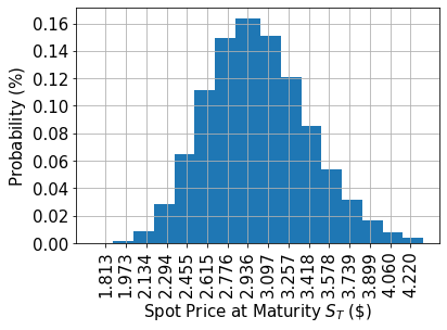
# plot probability distribution
x = uncertainty_model.values
y = uncertainty_model.probabilities
plt.bar(x, y, width=0.2)
plt.xticks(x, size=15, rotation=90)
plt.yticks(size=15)
plt.grid()
plt.xlabel("Spot Price at Maturity $$S_T$$ (\$)", size=15)
plt.ylabel("Probability ($\%$)", size=15)
plt.show()

# set the strike price (should be within the low and the high value of the uncertainty)
strike_price = 1.896

# set the approximation scaling for the payoff function
c_approx = 0.1

# setup piecewise linear objective fcuntion
breakpoints = [low, strike_price]
slopes = [0, 1]
offsets = [0, 0]
f_min = 0
f_max = high - strike_price
european_call_objective = LinearAmplitudeFunction(
    num_uncertainty_qubits,
    slopes,
    offsets,
    domain=(low, high),
    image=(f_min, f_max),
    breakpoints=breakpoints,
    rescaling_factor=c_approx,
)

# construct A operator for QAE for the payoff function by
# composing the uncertainty model and the objective
num_qubits = european_call_objective.num_qubits
european_call = QuantumCircuit(num_qubits)
european_call.append(uncertainty_model, range(num_uncertainty_qubits))
european_call.append(european_call_objective, range(num_qubits))


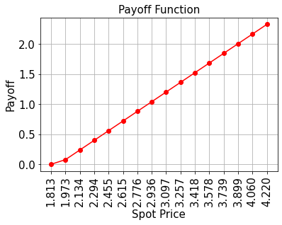
# plot exact payoff function (evaluated on the grid of the uncertainty model)
x = uncertainty_model.values
y = np.maximum(0, x - strike_price)
plt.plot(x, y, "ro-")
plt.grid()
plt.title("Payoff Function", size=15)
plt.xlabel("Spot Price", size=15)
plt.ylabel("Payoff", size=15)
plt.xticks(x, size=15, rotation=90)
plt.yticks(size=15)
plt.show()

# set target precision and confidence level
epsilon = 0.01
alpha = 0.05

qi = QuantumInstance(Aer.get_backend("aer_simulator"), shots=100)
problem = EstimationProblem(
    state_preparation=european_call,
    objective_qubits=[4],
    post_processing=european_call_objective.post_processing,
)
# construct amplitude estimation
ae = IterativeAmplitudeEstimation(epsilon, alpha=alpha, quantum_instance=qi)

conf_int = np.array(result.confidence_interval_processed)
print("Exact value:        \t%.4f" % exact_value)
print("Estimated value:    \t%.4f" % (result.estimation_processed))
print("Confidence interval:\t[%.4f, %.4f]" % tuple(conf_int))

Result:
Exact value:        	1.1162
Estimated value:    	1.1340
Confidence interval:	[1.1015, 1.1665]

### This code is a part of Qiskit. I did some modification to show some ideas.
In this qiskit example, we leverage a LinearAmplititudeFunction to translate \(f(i)\) into \(\tilde{f}(i)\) and the qiskit package would use post_processing to turn it back to real value.
Reference:
1. Nielsen, Michael A., and Isaac Chuang. "Quantum computation and quantum information." (2002): 558-559.
2. Asfaw, Abraham, et al. "Learn quantum computation using qiskit." Accessed: Oct 24 (2020): 2020.
3. Susskind, Leonard, and Art Friedman. Quantum mechanics: the theoretical minimum. Basic Books, 2014.
4. Rebentrost, Patrick; Gupt, Brajesh; Bromley, Thomas R. (2018): Quantum computational finance: Monte Carlo pricing of financial derivatives. In Phys. Rev. A 98 (2), p. 41. DOI: 10.1103/PhysRevA.98.022321.
5. Brassard, Gilles, et al. "Quantum amplitude amplification and estimation." Contemporary Mathematics 305 (2002): 53-74.
6. Stamatopoulos, Nikitas, et al. "Option pricing using quantum computers." Quantum 4 (2020): 291.
7. Y. Suzuki, S. Uno, R. Raymond, T. Tanaka, T. Onodera, and N. Yamamoto, “Amplitude estimation without phase estimation,” Quantum Inf Process, vol. 19, no. 2, p. 75, Feb. 2020, doi: 10.1007/s11128-019-2565-2.