1. Introduction
Given a set \(X = {0, 1, \ldots, N-1}\) and a boolean function \(\chi: X \longrightarrow {0, 1}\), we aim to find a good element, i.e., an \(x \in X\) such that \(\chi(x) = 1\).
A classical search algorithm has an average complexity of \(\sum_{i=1}^{N} i \times \frac{1}{N} = \frac{N + 1}{2}\) if there is only one good element. The quantum approach starts with an equal superposition of states \(\ket{\Psi} = \frac{1}{\sqrt{N}} \sum_{x=0}^{N-1} \ket{x}\). If we do not involve quantum algorithms, measuring \(\ket{\Psi}\) gives the correct \(\ket{x}\) with probability \(1/N\), so the average number of measurement is still \(\sum_{i=1}^{N} i \times \frac{1}{N} = \frac{N + 1}{2}\).
Grover’s algorithm transforms \(\ket{\Psi}\) in \(\mathcal{O}(\sqrt{N})\) iterations such that measuring it gives the correct \(\ket{x}\) with higher probability.
Amplitude amplification is a generalization of Grover’s algorithm where the input is an arbitrary superposition of elements of \(X: \ket{\Psi} = \mathcal{A} \ket{0} = \sum_{x \in X} \alpha_{x} \ket{x}\) and more than one element may be good state. We can write \(\ket{\Psi} = \sum_{x: \chi(x) = 1} \alpha_{x} \ket{x} + \sum_{x: \chi(x) = 0} \alpha_{x} \ket{x} = \ket{\Psi_{1}} + \ket{\Psi_{0}}\) with \(a = \left\langle \Psi_{1} \mid \Psi_{1} \right\rangle \ll 1\) being the probability of measuring \(\ket{\Psi}\) and obtaining a good state \(\mid \Psi_{1} \rangle\).
Therefore, the classical approach requires \(\mathcal{O}(1/a)\) iterations to find a good state, while amplitude amplification provides a quadratic speed-up in \(\mathcal{O}(\sqrt{1/a})\).
2. Review of Grover Search
The amplitude amplification operator \(Q\) is defined in terms of the oracle function \(S_{\chi}\), which maps the state \(\vert x\rangle\) to \(-\vert x\rangle\) if \(\chi(x)=1\) and to \(\vert x\rangle\) otherwise. The operator \(\mathcal{A}\) transforms the state \(\vert 0\rangle\) to the state \(\vert \Psi\rangle=\vert \Psi_{1}\rangle+\vert \Psi_{0}\rangle\). The oracle function \(S_{\chi}\) is defined as \(S_{\chi}=\frac{2}{1-a}\vert \Psi_{0}\rangle\langle\Psi_{0}\vert -I\). The operator \(S_{0}\) is defined as \(S_{0}=I-2\vert 0\rangle\langle 0\vert\). The amplitude amplification operator is then defined as
\[\begin{aligned} Q&= - \mathcal{A} S_0 \mathcal{A}^{\dagger} S_{\chi} = \left(\mathcal{A}(2\vert 0\rangle\langle 0\vert -I) \mathcal{A}^{\dagger}\right) S_{\chi} \\ &=(2\vert \Psi\rangle\langle\Psi\vert -I)\left(\frac{2}{1-a}\left\vert \Psi_{0}\right\rangle\left\langle\Psi_{0}\right\vert -I\right) \\ &=U_\Psi U_{\Psi_0} \end{aligned}\]
Then we have:
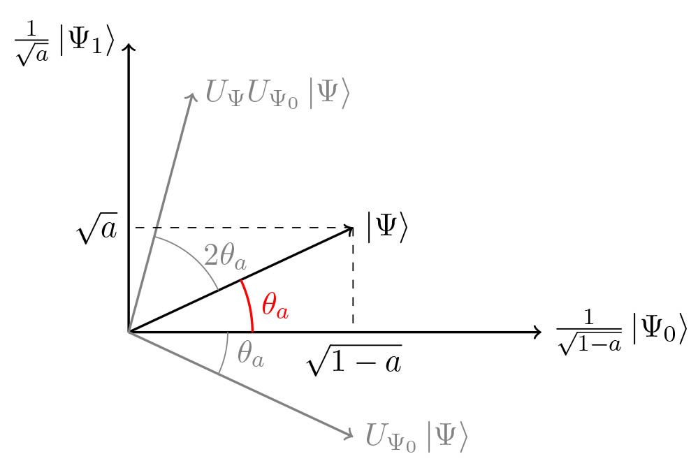
\[\begin{aligned} Q\left\vert \Psi_{1}\right\rangle &=U_{\Psi} U_{\Psi_{0}}\left\vert \Psi_{1}\right\rangle=-U_{\Psi}\left\vert \Psi_{1}\right\rangle=(I-2\vert \Psi\rangle\langle\Psi\vert )\left\vert \Psi_{1}\right\rangle \\ &=\left\vert \Psi_{1}\right\rangle-2 a\vert \Psi\rangle=(1-2 a)\left\vert \Psi_{1}\right\rangle-2 a\left\vert \Psi_{0}\right\rangle \\ Q\left\vert \Psi_{0}\right\rangle &=U_{\Psi}\left\vert \Psi_{0}\right\rangle=(2\vert \Psi\rangle\langle\Psi\vert -I)\left\vert \Psi_{0}\right\rangle \\ &=2(1-a)\vert \Psi\rangle-\left\vert \Psi_{0}\right\rangle=2(1-a)\left\vert \Psi_{1}\right\rangle+(1-2 a)\left\vert \Psi_{0}\right\rangle \end{aligned}\]Using the identity \(\sin^{2}(\theta_a)=a\) and \(\cos^{2}(\theta_a)=1-a\), we can derive the following:
\[\begin{aligned} Q\frac{\vert \Psi_{1}\rangle}{\sqrt{a}} &= (1-2a)\frac{\vert \Psi_{1}\rangle}{\sqrt{a}} - 2\sqrt{a(1-a)}\frac{\vert \Psi_{0}\rangle}{\sqrt{1-a}} \\ &= \left(1-2\sin^{2}(\theta_a)\right)\frac{\vert \Psi_{1}\rangle}{\sqrt{a}} - 2\cos(\theta_a)\sin(\theta_a)\frac{\vert \Psi_{0}\rangle}{\sqrt{1-a}} \\ &= \cos(2\theta_a)\frac{\vert \Psi_{1}\rangle}{\sqrt{a}} - \sin(2\theta_a)\frac{\vert \Psi_{0}\rangle}{\sqrt{1-a}} \\ Q\frac{\vert \Psi_{0}\rangle}{\sqrt{1-a}} &= \sin(2\theta_a)\frac{\vert \Psi_{1}\rangle}{\sqrt{a}} + \cos(2\theta_a)\frac{\vert \Psi_{0}\rangle}{\sqrt{1-a}} \end{aligned}\]Therefore, \(Q\) can be represented as a rotation matrix in the basis \(\frac{1}{\sqrt{a}}\vert \Psi_{1}\rangle, \frac{1}{\sqrt{1-a}}\vert \Psi_{0}\rangle\):
\(\)Q=\begin{pmatrix}
\cos 2\theta_a & \sin 2\theta_a
-\sin 2\theta_a & \cos 2\theta_a
\end{pmatrix}\(\)
The matrix \(Q\) has eigenvalues \(e^{2i\theta_a}\) and \(e^{-2i\theta_a}\), with corresponding eigenvectors \(\frac{1}{2}(1, i)\) and \(\frac{1}{2}(1, -i)\), which we can denote as \(\vert \Psi_{+}\rangle\) and \(\vert \Psi_{-}\rangle\), respectively.
The state \(\vert \Psi\rangle\) can be expressed in the \(Q\)-eigenvector basis as: \(\vert \Psi\rangle=\frac{-i}{2}\left(e^{i \theta_{a}}\left\vert \Psi_{+}\right\rangle-e^{-i \theta_{a}}\left\vert \Psi_{-}\right\rangle\right)\) Applying the operator \(Q^{j}\) to this state results in: \(Q^{j}\vert \Psi\rangle=\frac{-i}{2}\left(e^{(2 j+1) i \theta_{a}}\left\vert \Psi_{+}\right\rangle-e^{-(2 j+1) i \theta_{a}}\left\vert \Psi_{-}\right\rangle\right)\) Expressed in the original basis of \(\frac{1}{\sqrt{a}}\left\vert \Psi_{1}\right\rangle, \frac{1}{\sqrt{1-a}}\left\vert \Psi_{0}\right\rangle\): \(Q^{j}\vert \Psi\rangle=\sin \left((2 j+1) \theta_{a}\right) \frac{1}{\sqrt{a}}\left\vert \Psi_{1}\right\rangle+\cos \left((2 j+1) \theta_{a}\right) \frac{1}{\sqrt{1-a}}\left\vert \Psi_{0}\right\rangle\) Measuring the state $\vert \Psi\rangle$ after $m$ applications of the operator $Q$ produces a good state with a probability equal to \(\sin ^{2}\left((2 m+1) \theta_{a}\right)\). This probability is maximized when \(m=\left\lfloor\frac{\pi}{4 \theta_{a}}\right\rfloor\) and when the value of \(a\) is known. Additionally, \(\sin ^{2}\left((2 m+1) \theta_{a}\right) \geq 1-a\).
The algorithm has a complexity of \(2 m + 1\) applications of \(\mathcal{A}\) and \(\mathcal{A}^{\dagger}\), which is approximately equal to \(\mathcal{O}\left(\frac{1}{\sqrt{a}}\right)\). The success probability of the algorithm is close to 1, with an approximation of \(1 - a \approx 1\). To ensure the best results, \(\theta_{a}\) should be small enough such that the approximation \(\theta_{a} \approx \sin \left(\theta_{a}\right)=\sqrt{a}\) is valid.
3. Overall Circuit
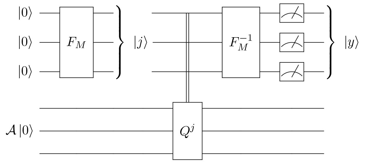
Then if we do not know \(\alpha\) in the first place, how can we find it?

Proof of correctness
The quantum circuit corresponds to the unitary transformation \(\left(F_{M}^{-1} \otimes I\right)\left(\Lambda_{M}(Q)\right)\left(F_{M} \otimes I\right)\) applied on the state \(\vert 0\rangle \otimes \mathcal{A}\vert 0\rangle\), with
\[\mathcal{A}\vert 0\rangle=-\frac{i}{\sqrt{2}}\left(e^{i \theta_{a}}\left\vert \Psi_{+}\right\rangle-e^{-i \theta_{a}}\left\vert \Psi_{-}\right\rangle\right)\]By applying \(F_{M} \otimes I\) :
\[\frac{1}{\sqrt{2 M}} \sum_{j=0}^{M-1}\vert j\rangle \otimes\left(e^{i \theta_{a}}\left\vert \Psi_{+}\right\rangle-e^{-i \theta_{a}}\left\vert \Psi_{-}\right\rangle\right)\]After applying \(\Lambda_{M}(Q)\) :
\[\frac{e^{i \theta_{a}}}{\sqrt{2}}\left\vert S_{M}\left(\theta_{a} / \pi\right)\right\rangle \otimes\left\vert \Psi_{+}\right\rangle-\frac{e^{-i \theta_{a}}}{\sqrt{2}}\left\vert S_{M}\left(1-\theta_{a} / \pi\right)\right\rangle \otimes\left\vert \Psi_{-}\right\rangle\]-
Finally, after \(F_{M}^{-1} \otimes I\), we have: \(\frac{e^{i \theta_{a}}}{\sqrt{2}} F_{M}^{-1}\left\vert S_{M}\left(\theta_{a} / \pi\right)\right\rangle \otimes\left\vert \Psi_{+}\right\rangle-\frac{e^{-i \theta_{a}}}{\sqrt{2}} F_{M}^{-1}\left\vert S_{M}\left(1-\theta_{a} / \pi\right)\right\rangle \otimes\left\vert \Psi_{-}\right\rangle\)
- By tracing out the second register in the eigenvector basis \(\left\vert \Psi_{+}\right\rangle,\left\vert \Psi_{-}\right\rangle\), we obtain a \(\frac{1}{2}-\frac{1}{2}\) mixture of \(F_{M}^{-1}\left\vert S_{M}\left(\theta_{a} / \pi\right)\right\rangle\) and \(F_{M}^{-1}\left\vert S_{M}\left(1-\theta_{a} / \pi\right)\right\rangle .\)
- By symmetry (since \(\sin ^{2}\left(\pi \frac{y}{M}\right)=\sin ^{2}\left(\pi\left(1-\frac{y}{M}\right)\right)\) ), we can assume the measured \(\vert y\rangle\) is the result of measuring \(F_{M}^{-1}\left\vert S_{M}\left(\theta_{a} / \pi\right)\right\rangle\).
- We thus have \(\tilde{\theta}_{a}=\pi \frac{y}{M}\) is a good estimate of \(\theta_{a}\) .
Bounding the error of the estimate \(\frac{1}{M} F_{M}^{-1}\left\vert S_{M}(\omega)\right\rangle\) is a good estimate of \(\omega\). Indeed, if \(\omega=x / M\) for some \(0 \leq x<M\), then \(F_{M}^{-1}\left\vert S_{M}(x / M)\right\rangle=\vert x\rangle\).
Otherwise: Theorem: Let \(X\) be the r.v. corresponding to the result of measuring \(F_{M}^{-1}\left\vert S_{M}(\omega)\right\rangle\). Then:
\[\mathbb{P}\left(\left\vert \frac{1}{M} X-\omega\right\vert \leq \frac{1}{M}\right) \geq \frac{8}{\pi^{2}} \approx 0.81\]Lemma: Letting \(\Delta=\left\vert \frac{1}{M} x-\omega\right\vert\) for some \(x \in 0, \ldots, M-1\), we have:
\[\mathbb{P}[X=x]=\frac{\sin ^{2}(M \Delta \pi)}{M^{2} \sin ^{2}(\Delta \pi)}\]Proof of the Lemma:
\[\begin{aligned} \mathbb{P}[X=x] &=\left\vert \left\langle x\left\vert F_{M}^{-1}\right\vert S_{M}(\omega)\right\rangle\right\vert ^{2} \\ &=\mid\left.\left(F_{M}\vert x\rangle\right)^{\dagger}\left\vert S_{M}(\omega)\right\rangle\right\vert ^{2} \\ &=\left\vert \left\langle S_{M}(x / M) \mid S_{M}(\omega)\right\rangle\right\vert ^{2} \\ &=\left\vert \left(\frac{1}{\sqrt{M}} \sum_{y=0}^{M-1} e^{2 \pi i x / M y}\langle y\vert \right)\left(\frac{1}{\sqrt{M}} \sum_{y=0}^{M-1} e^{2 \pi i \omega y}\vert y\rangle\right)\right\vert ^{2} \\ &=\frac{1}{M^{2}}\left\vert \sum_{y=0}^{M-1} e^{2 \pi i \Delta y}\right\vert ^{2}=\frac{\sin ^{2}(M \Delta \pi)}{M^{2} \sin ^{2}(\Delta \pi)} \end{aligned}\]Proof of the Theorem:
\[\begin{aligned} \mathbb{P}[d(X / M, \omega) \leq 1 / M] &=\mathbb{P}[X=\lfloor M \omega\rfloor]+\mathbb{P}[X=[M \omega]] \\ &=\frac{\sin ^{2}(M \Delta \pi)}{M^{2} \sin ^{2}(\Delta \pi)}+\frac{\sin ^{2}\left(M\left(\frac{1}{M}-\Delta\right) \pi\right)}{M^{2} \sin ^{2}\left(\left(\frac{1}{M}-\Delta\right) \pi\right)} \\ & \geq \frac{8}{\pi^{2}} \end{aligned}\]Since the minimum of this expression is reached at \(\Delta=1 /(2 M)\).
A bounding error on \(\tilde{\theta}_{a}\) translates into a bound on \(\tilde{a}\) . Lemma: Let \(a=\sin ^{2}\left(\theta_{a}\right)\) and \(\tilde{a}=\sin ^{2}\left(\tilde{\theta}_{a}\right)\) with \(0 \leq \theta_{a}, \tilde{\theta}_{a} \leq \frac{\pi}{2}\) . Then:
\[\left\vert \tilde{\theta}_{a}-\theta_{a}\right\vert \leq \epsilon \Longrightarrow\vert \tilde{a}-a\vert \leq 2 \epsilon \sqrt{a(1-a)}+\epsilon^{2}\]A bounding error on \(\tilde{\theta}_{a}\) translates into a bound on \(\tilde{a}\). Proof:
\[\begin{aligned} \tilde{a}-a=& \sin ^{2}\left(\tilde{\theta}_{a}\right)-\sin ^{2}\left(\theta_{a}\right) \leq \sin ^{2}\left(\theta_{a}+\epsilon\right)-\sin ^{2}\left(\theta_{a}\right) \\ =&\left(\sin \left(\theta_{a}\right) \cos (\epsilon)+\sin (\epsilon) \cos \left(\theta_{a}\right)\right)^{2}-\sin ^{2}\left(\theta_{a}\right) \\ =& \sin ^{2}\left(\theta_{a}\right) \cos (\epsilon)+\sin ^{2}(\epsilon) \cos ^{2}\left(\theta_{a}\right)+2 \cos \left(\theta_{a}\right) \sin \left(\theta_{a}\right) \cos (\epsilon) \sin (\epsilon) \\ &-\sin ^{2}\left(\theta_{a}\right) \\ =& \sin ^{2}(\epsilon)\left(\cos ^{2}\left(\theta_{a}\right)-\sin ^{2}\left(\theta_{a}\right)\right)+\sqrt{a(1-a)} \sin ^{2}(\epsilon) \\ =& \sqrt{a(1-a)} \sin (2 \epsilon)+(1-2 a) \sin ^{2}(\epsilon) \\ \leq & 2 \epsilon \sqrt{a(1-a)}+\epsilon^{2} \end{aligned}\]Same for \(a-\tilde{a}\).
Combining those results, the Amplitude Estimation algorithm outputs \(\tilde{\theta}_{a}\) such that
\[\begin{aligned} &\left\vert \tilde{\theta}_{a} / \pi-\theta_{a} / \pi\right\vert \leq \frac{1}{M} \\ &\Longleftrightarrow\left\vert \tilde{\theta}_{a}-\theta_{a}\right\vert \leq \frac{\pi}{M} \end{aligned}\]with probability greater than \(8 / \pi^{2}\). Thus, by setting \(\epsilon=\frac{\pi}{M}\) :
\[\vert \tilde{a}-a\vert \leq 2 \pi \frac{\sqrt{a(1-a)}}{M}+\frac{\pi^{2}}{M^{2}}\]Amplitude amplification when \(\alpha\) is not known
4. Application to Monte Carlo sampling
- Let \(X\) be a random variable taking values \(0, \ldots, N\) with probability \(p_{i}\). We want to compute \(\mathbb{E}[f(X)]\).
- Using Monte Carlo sampling, with \(M\) evaluations of \(f\), we get: \(\frac{1}{M} \sum_{k=0}^{M} f\left(X_{k}\right) \approx \mathbb{E}[f(X)] \pm \frac{C}{\sqrt{M}}\)
Quantum approach: define
\[\vert \Psi\rangle=\sum_{i=0}^{N-1} \sqrt{p_{i}}\vert i\rangle\]and the operator
\[F:\vert i\rangle \otimes\vert 0\rangle \mapsto\vert i\rangle \otimes(\sqrt{1-f(i)}\vert 0\rangle+\sqrt{f(i)}\vert 1\rangle)\]Then:
\[F\vert \Psi\rangle \otimes\vert 0\rangle=\sum_{i=0}^{N-1} \sqrt{1-f(i)} \sqrt{p_{i}}\vert i\rangle \otimes\vert 0\rangle+\sqrt{f(i)} \sqrt{p_{i}}\vert i\rangle \otimes\vert 1\rangle\]Using amplitude estimation, we estimate the probability to measure \(\vert 1\rangle\) in the last Qbit: \(\tilde{a}=\sum_{i=0}^{N-1} p_{i} f(i)=\mathbb{E}[f(X)]\), and using \(M\) evaluations of \(f\) :
\[\vert \tilde{a}-a\vert \leq 2 \pi \frac{\sqrt{a(a-a)}}{M}+\frac{\pi^{2}}{M^{2}}\]with a convergence rate of \(\mathcal{O}\left(\frac{1}{M}\right)\) to be compared to the classical \(\mathcal{O}\left(\frac{1}{\sqrt{M}}\right)\) rate.
5. QSearch Algorithm
To be updated.
Reference:
1. Nielsen, Michael A., and Isaac Chuang. "Quantum computation and quantum information." (2002): 558-559.
2. Asfaw, Abraham, et al. "Learn quantum computation using qiskit." Accessed: Oct 24 (2020): 2020.
3. Susskind, Leonard, and Art Friedman. Quantum mechanics: the theoretical minimum. Basic Books, 2014.